High-performance computing is not always intuitive. When you want to extract the absolute most from your code, you must understand how to use platform characteristics to your advantage. Sometimes, doing more work on the programmer’s part results in faster code.
All performance isn’t measured by the same criteria. It may mean different metrics in different programs, or different metrics in different parts of a single program. In one program we may be interested in getting the smallest possible response time (latency); in another, we may want the maximum possible amount of data transferred at once (throughput), and in yet another application we may simply be interested in making sure that if one instance of our program fails, another can take its place without a hitch (availability).

Above: Linux System Monitor showing several resource stats. Performance deals with several metrics.
The first pass for successful optimization is to figure out what matters most. More often than not, focus on that goal as two different optimization metrics may be completely incompatible. In fact, there is a saying in the area of distributed computing that says that, “Ideally, you want a system that is fast, always available, and scalable. But you can only pick two out of those.”
For the purposes of this article, I consider only performance when defined as doing computational work as fast as possible (i.e. execution speed). That tends to be the immediate performance problem a programmer deals with.
A note on premature optimization
Premature optimization is defined as trying to optimize a computer program that is still in its design phase. This has two main issues:
Performance optimization cycle
Initial performance optimization follows a predictable cycle:
- Write code.
- Run program.
- See that something seems to be way too slow (if you are lucky).
- Profile the program.
- Optimize code path.
- “Rinse and repeat” until satisfied.
- Profit!
Unfortunately for us, step 5 is a bit more involved than it looks when used in conjunction with the other steps in that list. Let’s try a very simple example to have an idea of how it would work.
Imagine the following C++ code snippet:
bool FullyContains(const int a[], int size_a, const int b[], int size_b) { for (int i = 0; i < size_b; ++i) { bool found = false;
for (int j = 0; j < size_a; ++j) { if (a[j] == b[i]) { found = true;
}
}
if (!found) return false;
}
return true;
}
There are some small optimizations to begin with. For example, we can break the inner loop immediately when we find that a[j] == b[i] (which is a good thing to do anyway), but in most cases these types of optimizations tend not to help much. We could also check if size_b < size_a and return earlier, but this can only be done if we know that the b array has no repeated numbers or that we don't allow multiple repeated numbers in the b array to match a single identical number in the a array. When profiling the code you figure out this code snippet runs very slowly for large array sizes (the complexity is O(N * M)).
Reducing the complexity always gives you the best bang for your buck. In our example, what if we could simply eliminate the inner loop (which also happens to be the larger one, most of the time)? Consider this new version of the same code:
bool FullyContains(const int a[], int size_a, const int b[], int size_b) { unordered_set<int> a_hash(a, a + size_a);
for (int i = 0; i < size_b; ++i) { if (a_hash.find(b[i]) == a_hash.end()) return false;
}
return true;
}
What we did here is copy our (usually larger) a array to a hash table. Then, instead of looping through all the entries in the a array, we simply do a lookup in this table (this operation is amortized O(1)). Actually copying the data from the array to the hash table is O(N) and is executed only once. The inner loop is also O(N), so our overall complexity turns up to be O(N).
Beyond the performance threshold
It is common, at some point during the performance optimization process, to reach a point where it seems we have optimized everything we could. But, unfortunately, we still have a performance-critical section that's taking more time than we wanted, and we are not sure why, as the operation it is doing seems trivial.
Let's consider the following code snippet (which is based on the canonical example for what we want to show):
long long GenerateSum(const int data[], int size_data) { long long sum = 0;
for (int i = 0; i < 100000; ++i) { for (int j = 0; j < size_data; ++j) { if (data[j] >= 128) { sum += data[j];
}
}
}
return sum;
}
For the sake of demonstration, let’s assume you tested this code with a sorted data array. Here are the results on your computer (this was obviously executed on my computer, but you get the idea): This function is pretty straightforward. It receives an array of ints and adds all of those that are equal to or greater than 128 (we only have values ranging from 0 to 255), repeating this operation 100,000 times. (Computers are way too fast these days, so we have to cheat a bit. Removing this loop and multiplying the result by 100,000 is not an optimization option in this case.) The code returns the accumulated sum.
time = 7.21
sum = 314931600000
But, then, when you ran it in production, you noticed it was a lot slower than expected! In fact, when profiling it with a real workload, you got something like this:
time = 22.65
sum = 314931600000
When comparing the data you used for testing originally and the data from production, you noticed they were exactly the same (as can be corroborated by the resulting sum). The only difference was that, in your test, you sorted the data first. But why would that matter, considering you did not optimize the code (at least not intentionally) for the case where arrays are sorted?
Welcome to the wonderful world of branch prediction
To understand what happened above, we must first understand what branch prediction is.
Modern computers are really fast. One of the ways they can be as fast as they are is by using the concept of instruction pipelines for code execution. Basically, the CPU fetches instructions from memory to one of its pipelines where they are executed as fast as possible. Pipelines work very well for serialized workflows, and can significantly increase the number of instructions that can be executed in one unit of time (thus increasing overall performance).
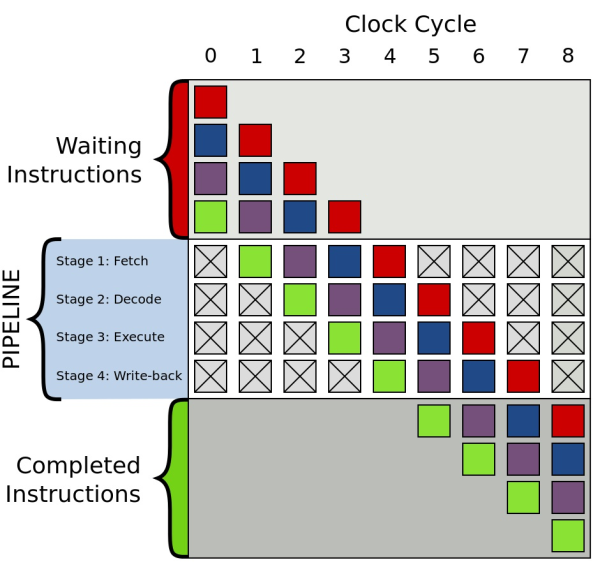 Above: Instruction pipeline representation. Blocks of different colors represent independent steps that can be executed at the same time (source: Wikipedia)
However, code usually has a lot of branches, so it can't be easily serializable. Whenever you hit a branch, you have to decide what way to go; you fetch the instructions for one branch or the other. If that were done randomly, there would be only a 50% chance of getting it right (assuming the probability of the input resulting in one branch or the other is 50%, of course).
Every time you get it wrong, the pipeline must be flushed and set up again with the correct instructions for the branch actually taken. That ends up being a very expensive operation. In fact, the CPU continues executing the wrong branch for a few cycles until it figures out that it took the wrong branch, and then the results are simply discarded.
To minimize the effects of selecting the wrong branch, pipelines are coupled with branch predictors that use different heuristics to try to correctly select the right branch most of the time. An example implementation of a branch predictor could keep a hit count for the frequency with which path of a branch is taken, such that the branch chosen is based simply on the path that currently has the higher count. This technique is usually referred to as a saturating counter.
By now, it should be clear what was happening in the example above. When the data contained in our array was in random order, the CPU successfully predicted the correct branch about 50% of the time, while it could do a significantly better job with sorted data.
So how could we solve this in our case? The simple approach is sort the array we get before running our loops (you should be seeing a pattern here by now). Another more interesting option is to write branchless code:
long long GenerateSum(const int data[], int size_data) { long long sum = 0;
for (unsigned int i = 0; i < 100000; ++i) { for (unsigned int j = 0; j < size_data; ++j) { unsigned long int temp = (data[j] - 128) >> 31;
sum += ~temp & data[j];
}
}
return sum;
}
With the change above, we removed the if condition (proof of how it works is left as an exercise for the reader). This has the advantage of not having to sort the array. It gives a good and predictable performance, with the disadvantage that reading the code now requires some amount of black magic.
Here is the result with an unsorted data array:
time = 6.51
sum = 314931600000
And with a sorted data array:
time = 7.56
sum = 314931600000
Keep in mind that this specific example was executed using GCC (with -O3). Intel has a compiler called ICC that, in this specific case, can convert the initial if check to code that is similar to the non-branch version above, so you get the optimization for free. Another option here is to use MMX/SSE, but this is outside the scope of this article.
Conclusion
Performance tuning is a really important part of every project, but it should be approached with the correct mindset. You must know your main objectives and have a solid design before trying to optimize. If you really need to make the best possible use of every CPU cycle available, you must have a good working knowledge of the particularities of the platform you are working on, and you must be prepared to deal with writing code that will not be easy to follow.
As a rule of thumb, don’t try to do deep optimization unless you really have to.
About the author:
Bruno Albuquerque is a technology addict with a passion for operating systems development. He worked as a kernel engineer for the Zeta OS and also as a contributor to the Haiku OS project. Currently he is a software engineer at Google.
See also: